V = confinement (pulls each particle toward center)Φ = interaction (between particles)σdW = random noise
Goal: learn V and Φ from unlabeled snapshots — without knowing which particle is which
The Setup
What are V and Φ?
Three particles under two forces. The blue arrows pull each particle toward the center (confinement V). The purple arrows push particles apart (interaction Φ). The gray arrows are random noise. The combined effect produces the complex motion you see.
We observe the particle positions, but we don't know V or Φ. Our goal: reverse-engineer these forces from the data alone.
The Problem
The Problem: Unlabeled Data
Imagine photographing a flock of birds at two different times. Each snapshot shows where every bird is — but you can't tell which bird is which across photos. Even with just 4 particles, there are 4! = 24 possible matchings. In real experiments with N=100, that's 100! ≈ 10158 — more than the atoms in the universe.
Toggle to see what information is lost
Left: labeled snapshot. Right: same particles, unknown identity. Which matching is correct?
Without labels, we cannot match particles across snapshots — and we don't try to. Our method works directly with the empirical distribution, bypassing the N! combinatorial explosion entirely.
The Challenge
Why Existing Methods Fail
Traditional methods estimate velocity as v ≈ ΔX/Δt. This creates two fatal problems: when Δt is small, noise explodes (∝ σ/√Δt); when Δt is large, discretization bias grows as O(Δt) and Sinkhorn matching accuracy drops to random chance. Drag the slider to see the collapse:
Prediction from §Solution: Self-test error is robust to large observation gaps Δt. Label-matching error explodes.
Labeled MLE: Noise Explosion
Estimates velocity as v ≈ ΔX/Δt. When Δt → 0, noise ∝ σ/√Δt → ∞. When Δt is large, O(Δt) discretization bias accumulates over N−1 interaction terms.
∇V: 0.8% → 11.3% as Δt grows
Sinkhorn MLE: Matching Collapse
Uses optimal transport to guess which particle is which. At small Δt, works well (particles barely move). At large Δt, particles mix completely — matching accuracy drops to 24.5%, near the 10% random baseline.
∇Φ: 0.8% → 95.8% as Δt grows
Our self-test avoids both pitfalls: no velocity estimation, no trajectory matching
Self-Test ∇V: 0.67% → 6.84%. In the same large-Δt benchmark row, Sinkhorn degrades much more severely.
But Approach 2 Also Fails
Distribution Matching: Correct Idea, Prohibitive Cost
Avoid labels entirely by minimizing Wasserstein distance between predicted and observed distributions. Sounds reasonable — BUT this requires simulating the full particle system at EVERY gradient step. For N=10 particles over 1000+ optimization steps, the compute cost explodes.
Drag to see how cost scales
Failure type: computational. Wasserstein minimization requires O(N² × optimization_steps) work — intractable for large systems.
And Approach 3 Also Fails
Mean-Field: Elegant Theory, Wrong Regime
For N→∞, the empirical measure converges to a smooth density satisfying a partial differential equation (PDE) — enabling clean inference. BUT: we care about finite N. At N=10, the empirical measure is 10 discrete delta spikes. Mean-field theory breaks down exactly here.
Drag N — observe when empirical measure becomes smooth enough for mean-field
Failure type: theoretical. Mean-field is valid only as N→∞. Our paper uses N=10. The approximation error from mean-field is O(1/N) — at N=10, this is 10% error before we've even started.
Three approaches. Three distinct failures. Time to ask a different question.
The Key Reframe
Stop Recovering What's Missing. Start From What We Have.
Every failed approach tried to RECOVER hidden information: labels, trajectories, or smooth density. None asked: what object do we ACTUALLY observe from unlabeled snapshots? And what can we build from THAT?
Phase 1: Labeled trajectories (classical setting)
This is the empirical measure μn = (1/N)∑i δXi. It is NOT a degraded version of trajectories. It is a different mathematical object — a random sum of N Dirac delta masses. And crucially: it has its own evolution equation.
Why This Formulation
The Observable Forces the Formulation
Pointwise Equation: Impossible
μn is a sum of delta spikes. Try ∂μn/∂x at a particle location: it's ∞. Pointwise derivatives don't exist for delta masses. We CANNOT write ∂tμn = ... in the classical sense.
Weak Form: The Only Path
∫ψ dμn = (1/N)∑i ψ(Xi). This is computable from any snapshot. Weak form turns the problem into: find (V,Φ) such that this empirical average matches the predicted evolution for all test functions ψ.
"We do not move to weak form because it is fancy. We move because the observable itself forces us to."
What Must Any Solution Satisfy?
Three Criteria for a Valid Test Family
Weak form reduces the problem to: choose a test function family ψ. But not any family works. Before we reveal the answer, check off each criterion that any valid family must satisfy.
The Self-Test Family: ψ = V + Φ*μ
Use the candidate potential ITSELF as the test function. This family satisfies all three criteria automatically: it's computable from μn, it's linear in (V,Φ), and it induces a well-structured (symmetric, non-negative) bilinear form. The self-test family is not a trick — it is the natural answer to the test-function design problem.
Our Approach
From Particles to Distributions: The Weak Form PDE
Key realization: we don't need to track individual particles. The empirical measure μtN = (1/N)∑iδX_t^i is directly observable from unlabeled snapshots. More importantly, it satisfies a weak-form stochastic evolution equation whose dependence on V and Φ is linear. This turns the N! matching problem into a functional optimization problem.
Why the Weak Form?
The empirical measure μtN satisfies a weak-form stochastic evolution equation. Because μtN is a sum of delta masses, its derivatives are understood distributionally rather than pointwise. The weak form handles this by testing the equation against a smooth function ψ and integrating by parts, so everything reduces to empirical averages over particle positions that are directly computable from snapshots.
Strong Form
Requires distributional derivatives of μ — not directly usable pointwise for delta masses
Weak Form
Only needs ∫ψ dμ = (1/N)∑ψ(Xᵢ) — computable!
Key Property
Linear in the unknown potentials → quadratic loss in the parametric setting
The crucial advantage: because the weak form PDE is linear in V and Φ, we can choose the test function ψ to be V and Φ themselves. This self-testing trick — using the unknowns as their own test functions — produces a loss with a remarkable property.
The Self-Test Loss
Applying Itô's formula with the self-testing family ψ = V + Φ*μ, the weak-form residual decomposes into three computable terms. The associated free-energy increment uses Ef(μ) = ⟨V + (1/2)Φ*μ, μ⟩. Each term is an empirical average over particle snapshots — no velocity estimation, no trajectory matching.
L(θ)=21JdissΔt−2σ2JdiffΔt+δEf
Anatomy of the Loss
Each term comes from testing the weak-form equation against ψ = V + Φ*μ. The last term is the free-energy increment associated with Ef(μ) = ⟨V + (1/2)Φ*μ, μ⟩:
Dissipation: how much work the drift forces do. The 1/2 coefficient (from the self-test trick) is what breaks the degeneracy — it makes L(V*, Φ*) strictly negative.
Jdiff = (1/N) ΣiΔV + (1/N²) Σi≠jΔΦ
Diffusion contribution: depends on the Laplacian of V and Φ. Computable from snapshots via the basis expansion or neural network parameterization.
δEf = Ef(t+Δt) − Ef(t)
For a candidate pair (V, Φ), the free-energy change between two unlabeled snapshots is computable without labels or trajectory matching.
Why Not Just Square the Residual?
Squaring the weak form residual creates a degenerate minimum at V=0, Φ=0 (the trivial solution). By contrast, the self-test loss gives the true potentials a strictly lower population loss than the trivial pair, which breaks that degeneracy.
Why Not Energy Balance?
One can derive a free-energy balance identity for the stochastic system via Itô's formula, together with a martingale term. But using the squared residual of that identity for estimation is still a bad objective: Jdiss is already quadratic in V and Φ, so squaring the balance produces a quartic, non-convex optimization problem.
Energy Balance Approach
Match the free-energy balance in expectation. Since Jdiss is already quadratic in V and Φ, squaring the residual yields a quartic, non-convex objective.
Our Self-Test (Variation Approach)
Test the weak-form PDE against ψ = V + Φ*μ. The resulting loss stays quadratic; under linear parameterization it reduces to a convex linear-system solve.
The demo below illustrates a free-energy balance identity. Near the ground-truth scales, the displayed terms nearly cancel. But turning that identity into an estimator would still require quartic optimization — exactly what the self-test avoids.
Interpretation guide: this panel is a diagnostic visualization of the free-energy balance, not the training objective itself. The estimator we actually optimize is the quadratic self-test loss above.
What This Buys Us
Five Freedoms From The Self-Test Loss
Each criterion the self-test family satisfies translates into a concrete freedom. These aren't abstract advantages — each one resolves a specific failure mode you've already seen.
Two Implementations
From Theory to Practice
The self-test loss is agnostic to how V and Φ are parameterized. We implement it two ways:
📐
Self-Test LSE
Expand V, Φ in known polynomial/exponential basis functions. Solve the resulting linear least-squares system in closed form — fast within the chosen basis, but it requires prior knowledge of the potential family.
✓Closed-form linear solve ×Needs known basis
🧠
Self-Test NN
Parameterize V, Φ with MLPs. Optimize via gradient descent — flexible, and it does not require a hand-specified oracle basis, but it still requires training and architectural assumptions.
✓No oracle basis needed ×Requires training
↓ Same self-test loss ↓
The loss is the common contribution, not the parameterization. The current paper proves estimator bounds in the parametric setting; the NN implementation is supported empirically.
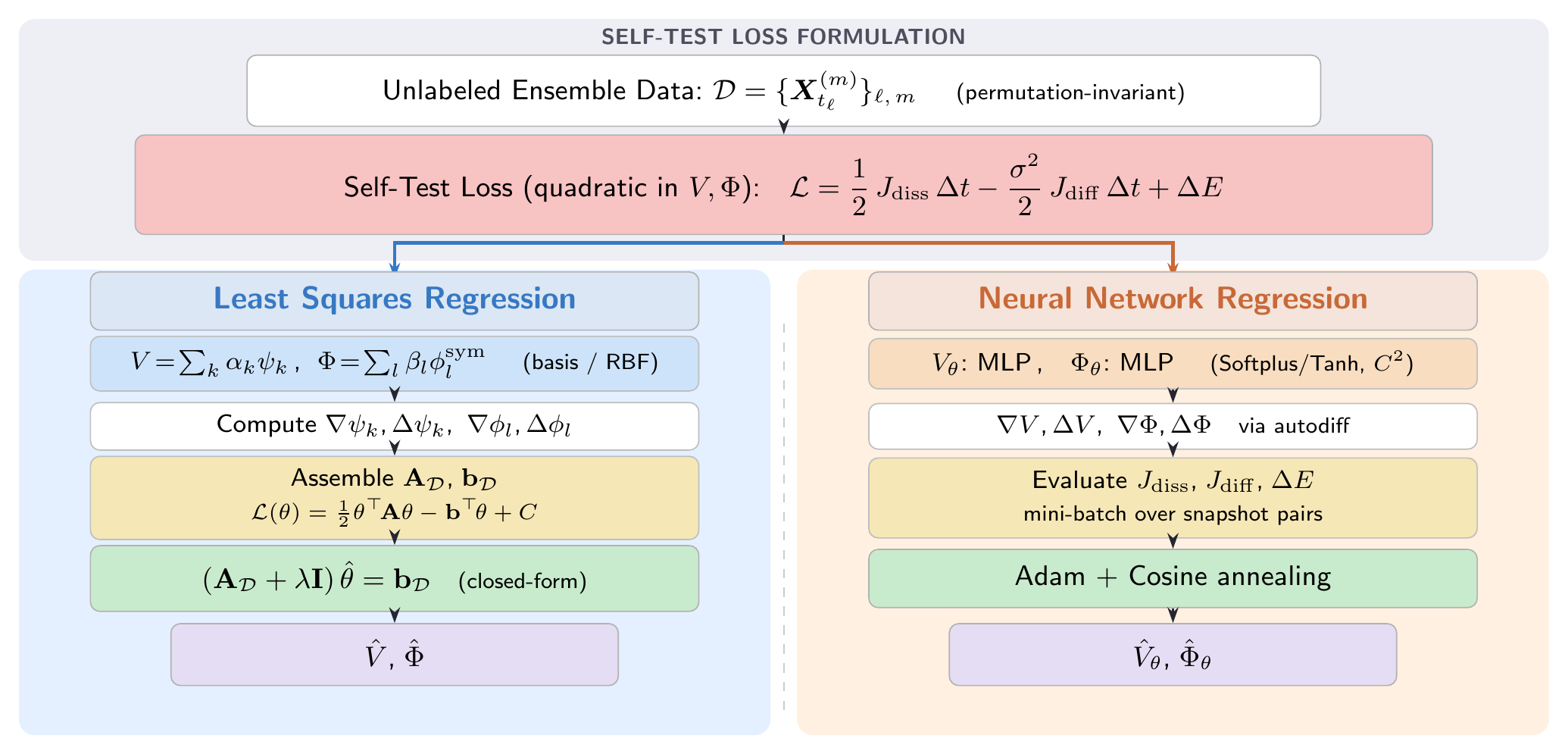
Figure 1: Algorithm Workflow
Left: Least squares regression with basis functions. Right: Neural network regression via gradient descent. Both share the same self-test loss.
Stress Tests
Reference + Four Boundary Tests
Reference model E serves as the main benchmark, while models A-D each probe one stressed assumption or difficult regime.
Note: potentials are identifiable only up to additive constants, so some displays use equivalent shifted forms with the same gradients. All quantitative errors reported below are gradient errors.
Potential Curves
Live Simulation (N=6)
Results by Model
Each model tests one theoretical assumption. Data at d=2, Self-Test LSE vs NN.
A: Smoothness Test
V=−21∣x∣+2∣x∣2,Φ=−3⋅1[0.5,1]ε+2⋅1[1,2]ε,ε=0.05
Smoothed-indicator Φ → stresses C⁴ smoothness
∇V: LSE 1.07% · NN 1.76%
∇Φ: LSE 2.01% · NN 3.32%
✓ Both handle non-smoothness well
B: Conditioning Test
V=41(∣x∣2−1)2−41,Φ=r+1γ
Inverse-type interaction → κ(A) = 146K, near-singular normal matrix
Shared protocol for all experiments. Reference model E (Gaussian Φ) satisfies all theoretical assumptions; models A-D each stress one boundary.
10
N particles
2–10
d dimensions
1.0
σ noise
2K
M snapshots
10−4
δt fine step
Theory Validation
Does the method work? Three questions.
Question 1: Does collecting more snapshots improve accuracy?
Yes. The error has two independent parts — a statistical part that shrinks with more data, and a discretization floor set by how far apart the snapshots are.
Statistical part: 1/√M
Collect more snapshot pairs M → error decreases as 1/√M. Double M → error drops ~30%.
Discretization floor: (Δt)^α
Set by the quadrature rule. α=1 (Riemann): floor ∝ Δt. α=2 (Trapezoidal): floor ∝ (Δt)². Once you hit this floor, more snapshots don't help.
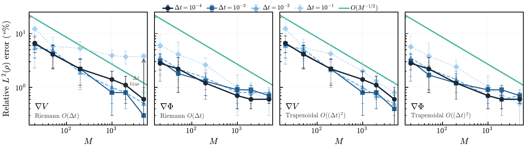
This figure verifies Q1: error ∝ 1/√M then hits the discretization floor.
Figure 2: M-scaling — Riemann vs Trapezoidal
Left: Riemann (α=1) — floor at O(Δt)
Error drops as 1/√M, then saturates.
Right: Trapezoidal (α=2) — floor at O((Δt)²)
Floor is quadratically lower — why we prefer the trapezoidal rule.
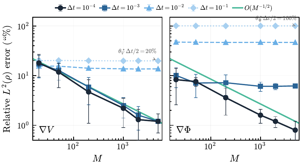
Question 2: What happens when snapshot pairs are far apart in time?
The discretization bias becomes intrinsic. When Δt = δt (zero gap), refining quadrature gives no extra benefit.
Figure 3: Discrete-Model Bias (zero-gap regime)
To push accuracy below O(Δt): use finer simulation (δt < Δt) and a higher-order quadrature rule.
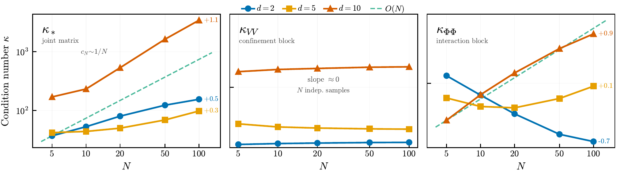
Question 3: Is the least-squares solve numerically stable?
Mostly yes. κ(A) grows at most as O(N) — the matrix stays controlled even as particle count grows.
d=2, Δt=10−2, M=2000, oracle basis. Theory predicts κ = O(N).
Model
N=5
N=10
N=20
N=50
N=100
Rate
E: Reference
37
53
80
123
155
0.5
A: Smoothness
42
46
88
208
396
0.8
B: Conditioning
81K
146K
262K
564K
962K
0.8
C: LJ
10.8K
12.1K
11.8K
12.1K
11.8K
0.0
D: Morse
7.9K
14.2K
25.4K
53.5K
89.5K
0.8
Figure 4: Condition Number Scaling with N
Three panels: κ* (total), κ_VV (V part, N-independent), κ_ΦΦ (Φ part, O(N)).
Reference model: κ = O(N⁰·⁵), well below O(N). Test B is the ill-conditioned outlier. LJ (C) has nearly constant κ driven by the r⁻¹² singularity.
Results
NN vs Basis: Who Wins?
The neural network knows nothing about the potential form, yet matches or beats the oracle basis in many settings. Below: Self-Test LSE vs Self-Test NN, all dimensions.
In our benchmarks, V is consistently easier to learn than Φ (NN ∇V < 5% in 15/16 settings), while Φ remains the bottleneck and is strongly model- and dimension-dependent. NN wins ∇V in 7/16 settings without knowing the potential form.
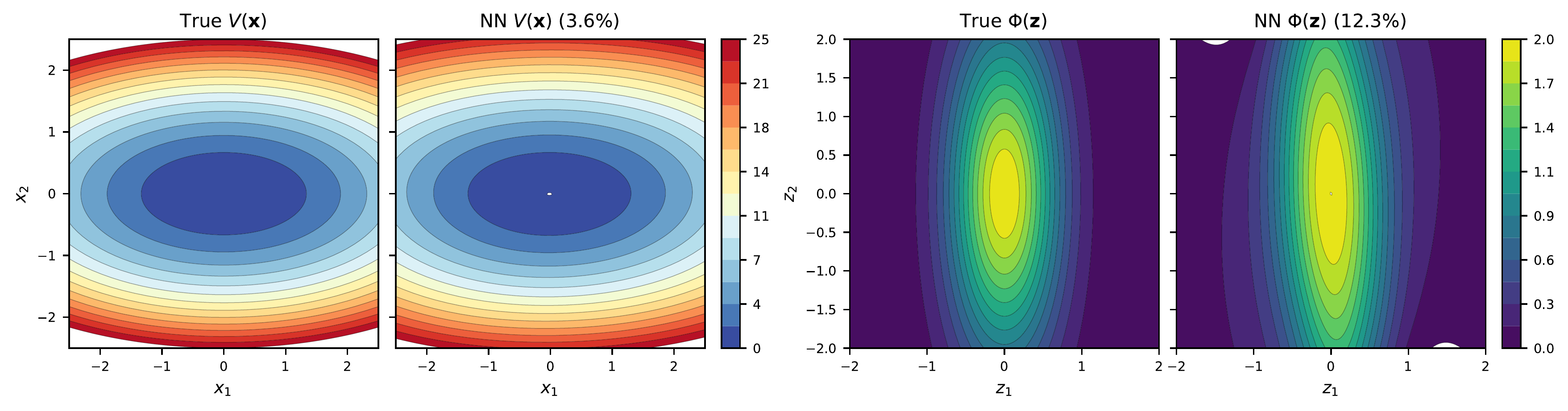
Figure 5: Non-Radial Potential Recovery (d=2)
The Non-Radial Model
External potential V(x)
V(x) = x₁² + 4x₂²
Elliptic confinement: 4× stronger along y-axis.
Interaction potential Φ(z)
Φ(z) = 2 exp(−½(z₁²/0.5² + z₂²/1.5²))
Direction-dependent interaction — range differs by axis.
Unlike all other test models, this Φ depends on direction — a harder case for the neural network.
All stress tests above use radial potentials V(|x|) and Φ(|z|). But real systems can be anisotropic — forces vary by direction. This figure tests whether the NN can recover non-radial potentials where each spatial axis has different parameters.
V(x): anisotropic confinement
a=(1,4) — 4× stronger along y-axis. NN recovers the elliptical shape with ∇V error 3.6%.
Φ(z): anisotropic interaction
Gaussian with s=(0.5, 1.5) — interaction range differs by axis. ∇Φ error 12.3%, harder due to pairwise coupling.
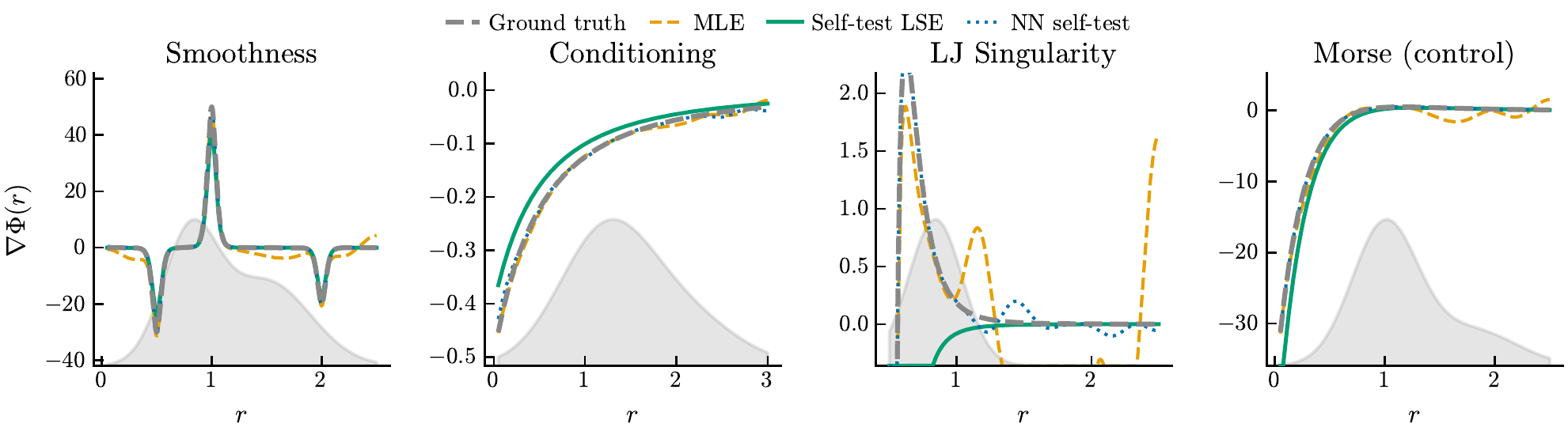
Figure 6: Boundary Recovery — Four Stress Tests
How well can we recover the interaction force Φ'(r) across different models? Each panel compares the true Φ' (black dashed) with LSE (green) and NN (blue) estimators. The gray shading shows the exploration measure ρΦ — where particles actually visit. Estimation quality degrades sharply outside the explored region.
Key insight: in these experiments, the gray exploration measure ρΦ is the dominant practical limitation. Both LSE and NN can only recover Φ' where data concentrates. Model C (Lennard-Jones) is the most extreme case: the r−12 singularity keeps particles apart, leaving the short-range force poorly resolved.
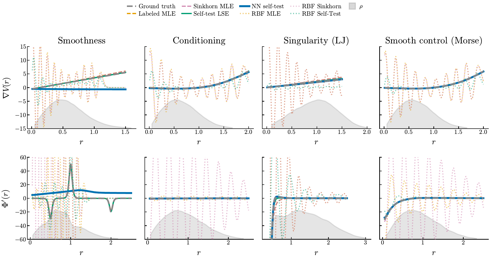
Figure 7: All Methods Comparison
The full picture: Self-Test (LSE and NN) vs Labeled MLE vs Sinkhorn MLE vs RBF basis, across all four stress-test models. Each row is one model; left column shows V', right column shows Φ'.
Self-Test (green/blue)
Tracks the target reasonably well in the tested models. NN is especially strong on V' because it does not rely on a hand-specified basis.
RBF basis (orange)
Produces oscillatory estimators — the wrong basis choice amplifies noise into spurious wiggles. This confirms why basis specification matters.
Regularization
The L-Curve: Automatic Regularization
Solving the basis regression (A + λI)x = b requires choosing the regularization parameter λ. Too small → noise amplified. Too large → solution over-smoothed. Hansen's L-curve is a heuristic selection rule: it picks the point of maximum curvature on the log-log trade-off curve between solution norm and residual norm.
The L-curve's characteristic ‘L’ shape emerges from two regimes: the vertical arm (small λ, noise dominates) and the horizontal arm (large λ, regularization bias dominates). The corner is often a useful operating point, but flat curves can make the heuristic fail. Try increasing the condition number to see how ill-conditioning sharpens the curve.
Deep Dive
The Mathematics
SDE Formulation
dXti=−∇V(Xti)−N1j=i∑∇Φ(Xti−Xtj)dt+σdWti
Each particle's motion is governed by three forces: confinement V, mean-field interaction Φ, and Brownian noise σ.
Applying Itô's formula to the free energy Ef(μ) = ⟨V + (1/2)Φ*μ, μ⟩ while testing the weak-form equation with ψ = V + Φ*μ. The 1/2 self-test coefficient arises from the variational construction, not from matching the free-energy balance directly.
Self-Test Loss Function
E[L(V∗,Φ∗)]=−21E[Jdiss∗Δt]<0vs.L(0,0)=0
The key innovation: the (1/2) coefficient on the dissipation term means L(V*, Φ*) = -(1/2) E[J_diss Δt] < 0, while L(0,0) = 0. This breaks the trivial-solution degeneracy.
Neural Network Architecture
Both V and Φ are parameterized by 3-layer MLPs with [64, 64, 64] hidden dimensions. The activation function must be C²-smooth (for example, Softplus or Tanh) — ReLU is not allowed because the self-test loss requires computing Laplacians via automatic differentiation, which needs second derivatives to exist. The symmetry Φ(x) = Φ(-x) is enforced architecturally. Total: ~17,000 parameters.