Skip to content

SpecViT

A systematic comparison of deep learning architectures for stellar surface gravity estimation

What attention learns from stellar spectra, where transformers help, and where hybrids still win

0.711
R² on DESI (50k)
0.196
MAE (dex)
0.098
σ on APOGEE

Key Findings

🎯

Near-Optimal at Low SNR

SpecViT comes within 0.02 R² of the Fisher Information / CRLB theoretical ceiling at SNR ≈ 4.6. The model extracts nearly all the information that is physically present in the data.

Clean Priors > Big Data

BOSZ-only training achieves σ = 0.098 on APOGEE, beating DESI-360k training (σ = 0.175) by 78%. Clean synthetic spectra provide more useful physical priors than massive noisy catalogs.

🔄

Cross-Survey Transfer

A single SpecViT model works across optical (DESI, 710–885 nm) and near-infrared (APOGEE, 1.5–1.7 μm) surveys. One architecture, multiple instruments.

The Challenge

Every star's light encodes its physical properties — gravity, temperature, composition. But extracting a single parameter (like surface gravity log g) from a noisy 4096-pixel spectrum is non-trivial, especially for faint targets at magnitude >20.

Key Insight: Not all wavelengths matter equally. Attention mechanisms can learn which spectral features are physically informative — the calcium triplet, magnesium lines, and iron features that carry the strongest gravity signal.

Interactive: SNR Degradation Explorer

Drag the slider to see how the same stellar spectrum degrades as the star gets fainter.

Method: Architecture Walkthrough

SpecViT applies Vision Transformer architecture to 1D stellar spectra:

Spectrum (4096 px) 256 Patches Token Embed 6-Layer ViT log g
SpecViT Architecture: Spectrum → Conv1D Patches → Transformer Encoder → log g prediction

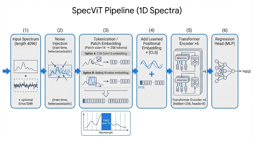
Interactive: Tokenization Visualizer

Hover over patches to see how the spectrum is divided. Patch colors show attention weight — brighter means higher attention.

Key Equations

Patch embedding:

Self-attention:

Training loss (Huber):

Attention Map Explorer

Explore what the model learns to attend to. The deepest layers concentrate attention on the Ca II infrared triplet (λ8498, 8542, 8662 Å) — the strongest surface gravity indicator in this wavelength range.

Static attention map (fallback) Averaged attention weights across 6 transformer layers, showing peaks at Ca II triplet wavelengths

Per-Head Attention Heatmap

Each attention head learns to focus on different spectral features. Head 1 specializes in the Ca II infrared triplet, while Head 5 captures positional patterns across the full wavelength range. Hover for details.

Results Dashboard

Explore SpecViT's performance across multiple axes. Click tabs to switch views.

Transfer Learning Story

How do synthetic spectra inform real-world prediction? We compare three strategies:

BOSZ Synthetic DESI Real APOGEE Test
Strategy Training Data σ (dex) MAE
BOSZ-only (Clean Prior) 50k BOSZ 0.098 0.956 0.071
DESI Direct 360k DESI 0.175 0.889 0.128
Two-Stage BOSZ + DESI 0.112 0.942 0.082
Key Insight: More data ≠ better. Clean synthetic priors (50k BOSZ) outperform massive noisy catalogs (360k DESI) by 78% in prediction scatter. Quality of physics modeling trumps quantity of observations.

Spectrum Explorer

Browse 7 example DESI spectra spanning giants, subgiants, and dwarfs. Drag to pan, scroll to zoom.

Performance by Stellar Type

SpecViT maintains consistent low MAE across stellar evolutionary stages — giants, subgiants, and dwarfs — while LightGBM struggles most with evolved stars where spectral features are subtler.

Deep Dive

Fisher Information & CRLB

The Cramér-Rao Lower Bound (CRLB) defines the minimum achievable variance for any unbiased estimator. For a parameter θ estimated from data x with likelihood p(x|θ):

We compute Fisher information from BOSZ synthetic spectra, where the noise model is known exactly. This gives us a theoretical performance ceiling against which we benchmark SpecViT.

Training Procedure

SpecViT-S (Small) configuration:

  • 6 Transformer layers, 6 attention heads, embed_dim = 384
  • Patch size = 16, num_patches = 256
  • AdamW optimizer, lr = 3e-4, cosine annealing
  • Huber loss (δ = 0.5), batch size = 256
  • Training: ~50 epochs on 1× A100 GPU (~30 min)
Computational Cost
Model Params Train Time Inference
Ridge Regression 4K <1 min <1 ms 0.507
LightGBM ~100K ~2 min <1 ms 0.647
SpecViT-S 7.4M ~30 min ~2 ms 0.731